MySQL Comparing INTs and CHARs

     How does MySQL compare INTs with CHARs? I was asked this very question over the weekend and wanted to share that information plus some of the changes in MySQL 8.0.21 in this area.  And yes those changes are pretty big.

Casting

    Computers are good at making comparisons of two values but only if everything else the same.  Comparing an integer with another integer is simple.  Same data with same data type comparisons are a good thing.  But what about when you need to compare a numeric 7 with a "7" where the number is in a string?  In such cases one or both numbers need to be changed into the same basic data type. Imagine your favorite Harry Potter character waving their magic wand and shouting 'accio data' to change two different magical pieces of data into one common data type.  No, Hogwarts was the the reason this conversion is called casting but this 'magic' needs to be made for a good comparison.

    If you read the Optimizer Notes section of the MySQL 8.0.21 Release Notes you will run into a notice that MySQL injects casts to avoid mismatches for numeric and temporal data with string data. The big trick was keeping backward compatibility with previous versions while matching the SQL standard.  Now when the optimizer is comparing numeric and temporal types and the expected data type does not match  it will now add casting operations in the item tree inside expressions and conditions. For instance if you are comparing a YEAR to string they will both be converted to a DOUBLE.

Example

    We have two tables and are comparing an INT to a CHAR.  If we run EXPLAIN ANALYZE of the query we get the details.

explain analyze select * 
from t1 
join t2 on t2.k = t1.k\G

*************************** 1. row ***************************

EXPLAIN: -> Inner hash join (cast(t2.k as double) = cast(t1.k as double))  (cost=4.75 rows=5) (actual time=1.759..1.771 rows=5 loops=1)

    -> Table scan on t1  (cost=0.22 rows=6) (actual time=1.670..1.677 rows=6 loops=1)

    -> Hash

        -> Table scan on t2  (cost=0.75 rows=5) (actual time=0.034..0.043 rows=5 loops=1)

    If we look at the original query we are trying to join two tables where the CHAR t2.k is equal to the INT t1.k.   The magenta highlighted text above shows where both the t2.k and the t1.k columns are cast as doubles.

    Running EXPLAIN without the ANALYZE we can see the query plan's version of the query that has been generated by the optimizer.

explain select * from t1 join t2 on t2.k = t1.k\G
*************************** 1. row ***************************
           id: 1
  select_type: SIMPLE
        table: t2
   partitions: NULL
         type: ALL
possible_keys: NULL
          key: NULL
      key_len: NULL
          ref: NULL
         rows: 5
     filtered: 100
        Extra: NULL
*************************** 2. row ***************************
           id: 1
  select_type: SIMPLE
        table: t1
   partitions: NULL
         type: ALL
possible_keys: NULL
          key: NULL
      key_len: NULL
          ref: NULL
         rows: 6
     filtered: 16.666667938232422
        Extra: Using where; Using join buffer (hash join)
2 rows in set, 1 warning (0.0010 sec)
Note (code 1003): /* select#1 */ select `demo`.`t1`.`id` AS `id`,`demo`.`t1`.`k` AS `k`,`demo`.`t2`.`id` AS `id`,`demo`.`t2`.`k` AS `k` from `demo`.`t1` join `demo`.`t2` where (cast(`demo`.`t2`.`k` as double) = cast(`demo`.`t1`.`k` as double))

    We can see that the original query of select * from t1 join t2 on t2.k = t1.k has been rewritten to select `demo`.`t1`.`id` AS `id`,`demo`.`t1`.`k` AS `k`,`demo`.`t2`.`id` AS `id`,`demo`.`t2`.`k` AS `k` from `demo`.`t1` join `demo`.`t2` where (cast(`demo`.`t2`.`k` as double) = cast(`demo`.`t1`.`k` as double)) by the optimizer.  

    I highly recommend looking at the query plan to help understand what the MySQL server needs to do to make your query work.  

What Is The Difference Between GROUP BY and Windowing Functions? PART II

     Last time we covered the basic differences between GROUP BY and Windowing functions. We ended up with this query:

select distinct count(ID) over (partition by District) as count, 
    CountryCode, 
    count(CountryCode) over (partition by District) as '#', 
    District, 
    SUM(Population) over (partition by District)  as 'Pop City',        SUM(Population) over (partition by CountryCode) as 'Pop Country' from city 
where CountryCode IN ('USA','BEL') 
order by CountryCode,District;

    Which I admit is a little messy. We have three windows over rows with two separate qualifiers.  One of the nice things about Windowing Functions is that they clean up so nicely and also make them easier to read. What we need to do is break out the 'over (...) ' sections.  Let us call the 'partition by District' as D_win and partition by CountryCode as C_win.  

select distinct count(ID) over D_win as count, 
    CountryCode, 
    count(CountryCode) over D_win as '#', 
    District, 

    SUM(Population) over D_win  as 'Pop City', 
    SUM(Population) over C_win  as 'Pop Country' 
from city 
where CountryCode IN ('USA','BEL') 
window C_win as (partition by CountryCode),
D_win as (partition by District)
order by CountryCode,District;

    This is much easier to comprehend and will be much easier to modify.  

GROUP BY and ORDER BY Mutually Exclusive No More!

    Now back to GROUP BY.  

    Prior to MySQL 8.0.12 there was something a few folks tripped over - you cannot also use an ORDER BY clause to sort the results. In other words, ROLLUP and ORDER BY were mutually exclusive in MySQL. But this as changed in '12 and you can no send queries like this:

select region, 

    count(name) as '# counties'  

from country 

group by Region with rollup 

order by Region;

+---------------------------+------------+

| region                    | # counties |

+---------------------------+------------+

| NULL                      |        239 |

| Antarctica                |          5 |

| Australia and New Zealand |          5 |

| Baltic Countries          |          3 |

| British Islands           |          2 |

| Caribbean                 |         24 |

| Central Africa            |          9 |

| Central America           |          8 |

| Eastern Africa            |         20 |

| Eastern Asia              |          8 |

| Eastern Europe            |         10 |

| Melanesia                 |          5 |

| Micronesia                |          7 |

| Micronesia/Caribbean      |          1 |

| Middle East               |         18 |

| Nordic Countries          |          7 |

| North America             |          5 |

| Northern Africa           |          7 |

| Polynesia                 |         10 |

| South America             |         14 |

| Southeast Asia            |         11 |

| Southern Africa           |          5 |

| Southern and Central Asia |         14 |

| Southern Europe           |         15 |

| Western Africa            |         17 |

| Western Europe            |          9 |

+---------------------------+------------+

    The reader of the output still has to know that the NULL entry under the region column is the rolled up total. And a lot of casual readers will be confused by having the total on the first line instead of the traditional placement on the last time. Now you can get the total on the bottom by adding DESC to the ORDER BY clause but now the regions are not ascending alpha order.  Dang trade offs.

    One thing to note is the query cost for the GROUP BY version is 264.40  (and yes these timing are relative to my hardware and should only be used for rough comparisions)

    But lets look at a Windowing Function version of this query:

select  distinct Region, 

        count(Name) over (partition by Region) 

from Country 

order by Region;

    The query cost here is 503.40!  Ouch!  The sort cost alone is 239.0! But Windowing Functions let you move the ORDER BY clause.

select    distinct Region, 

          count(Name) over (partition by Region order by Region) 

from Country;

    And the query cost is again 264.40. Yup, the same as the GROUP BY version.

    We do not have the ROLLUP functionality but as you saw in the last blog that it would not be hard to add.  First let us clean up the window definition.

select distinct Region,    

       count(Name) over w1 

from Country 

window 

    w1 as (partition by Region order by Region);

    Then add a new window definition:

select distinct Region, 

       count(Name) over w1, 

       count(Name) over w2 

from Country 

window 

    w1 as (partition by Region order by Region), 

    w2 as ();

    And the query cost is still 264.40.  

What Is The Difference Between GROUP BY and Windowing Functions? PART I

    I had an question that made me stop in my tracks -- What Is The Difference Between GROUP BY and Windowing Functions?  At one level there is a big difference and at another they are similar, at least in a few respects.

Definitions

    GROUP BY is described as "The GROUP BY statement groups rows that have the same values into summary rows, like "find the number of customers in each country". Another source says Window functions belong to a type of function known as a ‘set function’, which means a function that applies to a set of rows. The word ‘window’ is used to refer to the set of rows that the function works on.

    So both work on sets of rows. But what are the differences?

    Lets start with a goal and for the first example we want to know how many cities are in each District (or state) in the world.city table where the CountryCode = 'USA'. And lets write one query that uses GROUP BY and one query that uses a Windowing Function.  This query will be expanded to include more data just like queries expanded by the 'hey, this is nice but can you also get me ...' method.

Example Queries

    An example using GROUP BY

select count(id), 

       District 
from city 
where CountryCode='usa' 
group by District;

    And an example using a Windowing Function.  If you are unfamiliar with windowing functions the key word to look for is OVER(). 

select distinct count(ID) over (partition by District), 
    District  
 from city 
 where CountryCode='USA';

    Not too much of a difference. What about the query plan?  Using EXPLAIN FORMAT=JSON reveals the query cost is 102.4 for the GROUPY BY and 276.4 for the Windowing Function.  

 Which Query to Use?!?!

    I have always used the Occum's Razor rule when confronted with two equivalent queries and picked the simpler of the two. But while visually these took look similar the performance of the GROUP BY is appreciably better. 

WITH ROLLUP or OVER()??

    So lets make the query work a little harder.  Now we want a total off all the IDs counted and with the GROUP BY version we add WITH ROLLUP.

select count(id), 

        District 
from city 
where CountryCode='usa' 
group by District WITH ROLLUP;

    And at the very end of the output we see the number 274 (the number of rows) and NULL as the name of the district used for the rollup. And yes you are not only stuck with the district name of NULL but explaining that it is a place holder to those wanting this data.  

    The Windowing Function version's output is not as pretty as it adds a repeating column of '274' to each row of output. The difference is now a selection of count(id) over() to the query.

select distinct count(ID) over (partition by District), 

                count(ID) over(), 

District 
from city 
where CountryCode='USA';

    A bit of explanation is needed here.  There are now two Windowing Functions being used in this query.  The first count(ID) is partitioned by the District column while the second, with the empty parens, is not partitioned -- it is counting all the records.

Now Add the Population

    Now let's us pretend we like our queries but now we want to add the sum of the Population column for each district.

select count(id), 
        District, 
        sum(Population) as Pop 
       from city 
        where CountryCode='usa' 
        group by District, Population with rollup

                    limit 5;

    Please note that I am limit the output to ten rows to save the length of this blog from the horrendous level.  Here the GROUP BY has prioritized Population over District and the results are not exactly usable. We are getting the population rolled up for each state but it is probably not obvious at first glance.

+-----------+----------+--------+

| count(id) | District | Pop    |

+-----------+----------+--------+

|         1 | Alabama  | 158216 |

|         1 | Alabama  | 198915 |

|         1 | Alabama  | 201568 |

|         1 | Alabama  | 242820 |

|         4 | Alabama  | 801519 |

|         1 | Alaska   | 260283 |

|         1 | Alaska   | 260283 |

|         1 | Arizona  | 108364 |

|         1 | Arizona  | 109697 |

|         1 | Arizona  | 158625 |

+-----------+----------+--------+

  So lets switch the group by to 'GROUP BY Population, District' to prioritize Population. And what we get is not much better. The count of the cities in the individual districts is gone.  We are not getting the population sum by District with the ROLLUP but the output is not what we want.

+-----------+----------------+-------+

| count(id) | District       | Pop   |

+-----------+----------------+-------+

|         1 | South Carolina | 89063 |

|         1 | NULL           | 89063 |

|         1 | California     | 89089 |

|         1 | NULL           | 89089 |

|         1 | Texas          | 89293 |

|         1 | NULL           | 89293 |

|         1 | Illinois       | 89408 |

|         1 | NULL           | 89408 |

|         1 | Wisconsin      | 89447 |

|         1 | NULL           | 89447 |

+-----------+----------------+-------+

       GROUP BY can prioritize what we group the data by but as you see above it is limited by the mechanics of its definition. So we can very quickly outgrow GROUP BY.

Defenestration

    Windowing Function let you have a little more control over the results.  In the follow example we count the number of IDs per each District and sum the population for each District.      

select distinct count(ID) over (partition by District) as count,            District, 

        SUM(Population) over (partition by District)  as 'Pop' 

from city 

where CountryCode='USA' 

limit 10;

+-------+----------------------+----------+
| count | District             | Pop      |
+-------+----------------------+----------+
|     4 | Alabama              |   801519 |
|     1 | Alaska               |   260283 |
|     9 | Arizona              |  3178903 |
|     1 | Arkansas             |   183133 |
|    68 | California           | 16716706 |
|     9 | Colorado             |  1851149 |
|     5 | Connecticut          |   609087 |
|     1 | District of Columbia |   572059 |
|    15 | Florida              |  3151408 |
|     6 | Georgia              |  1148875 |
+-------+----------------------+----------+

    But let us expand the query to include two countries with the goal of getting the per district and per country information included.

select distinct count(ID) over (partition by District) as count, 

        CountryCode, 

        count(CountryCode) over (partition by District) 

               as 'Cities in District',             

        District, 

        SUM(Population) over (partition by District)  as 'Pop' 

from city 

where CountryCode IN ('USA','BEL') 

order by CountryCode,District 

limit 10;
+-------+-------------+--------------------+---------------+---------+
| count | CountryCode | Cities in District | District      | Pop     |
+-------+-------------+--------------------+---------------+---------+
|     1 | BEL         |                  1 | Antwerpen     |  446525 |
|     2 | BEL         |                  2 | Bryssel       |  239551 |
|     1 | BEL         |                  1 | East Flanderi |  224180 |
|     2 | BEL         |                  2 | Hainaut       |  291762 |
|     1 | BEL         |                  1 | Liège        |  185639 |
|     1 | BEL         |                  1 | Namur         |  105419 |
|     1 | BEL         |                  1 | West Flanderi |  116246 |
|     4 | USA         |                  4 | Alabama       |  801519 |
|     1 | USA         |                  1 | Alaska        |  260283 |
|     9 | USA         |                  9 | Arizona       | 3178903 |
+-------+-------------+--------------------+---------------+---------+

    Now we are partitioning by District over three separate pieces of data.  If we need to add another column for the sum of the population of each country, it is simple addition to the query. We do have to specify a new partitioning factor as now we need to group the rows for the new calculation accordingly.  Unlike using GROUP BY, there is no ambiguity on what is being prioritized. And we are getting the data the way we want.

select distinct count(ID) over (partition by District) as count,            CountryCode,     

        count(CountryCode) over (partition by District) as '#',            District, 

        SUM(Population) over (partition by District)  as 'Pop City',         SUM(Population) over (partition by CountryCode) 

            as 'Pop Country' 

from city 

where CountryCode IN ('USA','BEL') 

order by CountryCode,District 

limit 10;
+-------+-------------+---+---------------+----------+-------------+
| count | CountryCode | # | District      | Pop City | Pop Country |
+-------+-------------+---+---------------+----------+-------------+
|     1 | BEL         | 1 | Antwerpen     |   446525 |     1609322 |
|     2 | BEL         | 2 | Bryssel       |   239551 |     1609322 |
|     1 | BEL         | 1 | East Flanderi |   224180 |     1609322 |
|     2 | BEL         | 2 | Hainaut       |   291762 |     1609322 |
|     1 | BEL         | 1 | Liège        |   185639 |     1609322 |
|     1 | BEL         | 1 | Namur         |   105419 |     1609322 |
|     1 | BEL         | 1 | West Flanderi |   116246 |     1609322 |
|     4 | USA         | 4 | Alabama       |   801519 |    78625774 |
|     1 | USA         | 1 | Alaska        |   260283 |    78625774 |
|     9 | USA         | 9 | Arizona       |  3178903 |    78625774 |
+-------+-------------+---+---------------+----------+-------------+

    This is just scratching the surface of how and when to use Windowing Functions over GROUP BY and just skims the surface of the power of Windowing Functions (and yes, you can neaten things up from the examples). I hope to show in a future post some more of this power.

   

Two MySQL 8.0 Talks this week - DevOps and Features, an upcoming Podcast, and an article on JSON Document Validation

 I have two talks this week on MySQL 8.0 that you can attend virtually. And another session that is one line also plus an article.  Busy week!

First is a follow on to a earlier session I did for the good folks at cPanel want you to register here for MySQL 8.0 changes for DBAs and DevOps on August 12th, 2020  at 2PM CDT. The first talk was mainly for developers and this time I am, heavily covering InnoDB Cluster and features that are of more interest to the folks who keep MySQL instances running.

MergePHP - New MySQL Features That You May Have Missed is on Thursday August 13th at 7:00 Eastern . This is an exciting combination of three MySQL user groups who have joined together for a virtual meeting.

Then on Friday the 14th I am panelist for the JavaScript and Friends conference's panel on keeping your skills relevant in a changing world.

The gold folks at PHP Architect have published and article I

wrote on JSON Document Validation with MySQL  and we are getting setup for me to speak on their podcast on just that subject. 

MySQL InnoDB Cluster, MySQL NDB Cluster, and MySQL Replica Set

    MySQL has had replication for decades but the various options can be confusing.  One social media post I read recently could be summarized with the statement 'there are too many good options but how do I know which is right for me?'

Cluster

    Of all the words used in the computer related world, 'cluster' is the one that I wish we could have found a replacement for as the confusion over the word has created it's own cluster. Since MySQL has InnoDB Cluster and NDB cluster with other vendors using the word we end up with a lot of confusion. Add in clustered indexes and other non replication uses of the word to add more confusion. So which is what and where do we apply then for best performance.

MySQL Replication 101

    The follow is an overview of MySQL replication offerings and the details are in the manual.  And of course there are third party software that are not covered here that may have some utility for you. But so many folks are popping up on social media wanting a 'low cost five nines solution (99.999% up time)' solution or 'want to replicate terabytes of data to servers located around the world with automatic, sub-second fail over' that I thought it would be best to provide this overview.

    Imagine you have two servers with exact copies of the same data on their hardware.  One machine called the primary gets a query with an update/delete/modification and processes that query.  Part of the processing is writing the query (or the results of the query) to a file that the other system, called the replica, copies to its hardware and then applies to its copy of the data.  The end result is that once again both servers again have exact copies of the data.  

    Simple? Easy-peasy? Well then imagine adding in several thousand queries, network latency, differing work loads on the replica, and dozens of other issues that could impact performance. This imaginary situation provides a lot of queries and activities for both servers to juggle.  Just like a busy short order cook, it is possible for orders to get lost or scheduled poorly which in turns leads to unhappy customers.

    There are many ways to manage all this traffic, replication overhead, and administration.  

Simple Replication

    Replication enables data from one MySQL database server, known as a source or primary, to be copied to one or more MySQL database servers known as replicas. Replication is asynchronous by default but there is a semi-synchronous option.  The replicas do not need to be connected permanently to receive updates from a source. And you can configure replication to copy  all databases, selected databases, some databases of your choosing, or even selected tables within a database.

    This is a great way to scale out read traffic, provide a copy of the data for use with backups, or provide a copy of the data for development/test/analytics. The traditional method replicating events from the source's binary log, and requires the log files and positions in them to be synchronized between the source and the replica. A newer method uses global transaction identifiers (GTIDs) and is transactional, therefore it does not require working with log files or positions within these files, which greatly simplifies many common replication tasks. Replication using GTIDs guarantees consistency between source and replica as long as all transactions committed on the source have also been applied on the replica. And GTID based replication is easier to automate.

    MySQL supports three types of synchronization. The original type of synchronization is one-way, asynchronous replication, in which one server acts as the source and one or more other servers act as replicas. This is in contrast to the synchronous replication which is a characteristic of NDB Cluster which is covered later. MySQL 8.0's semisynchronous replication is in addition to the built-in asynchronous replication where a commit is performed on the source blocks before returning to the session that performed the transaction until at least one replica acknowledges that it has received and logged the events for the transaction

    There are two core types of replication format, Statement Based Replication (SBR), which replicates entire SQL statements, and Row Based Replication (RBR), which replicates only the changed rows. You can also use a third variety, Mixed Based Replication (MBR).  For the future it is best to row based replication which has the benefit of only sending the changes to the replicas instead of the query which can reduce traffic size.

NDB Cluster 

    You cell phone provider probably uses NDB (Network Data Base) cluster to track your phone's position relative to the nearest cell tower.  Wikipedia says MySQL Cluster is a technology providing shared-nothing clustering and auto-sharding for the MySQL database management system. It is designed to provide high availability and high throughput with low latency, while allowing for near linear scalability.[3] MySQL Cluster is implemented through the NDB or NDBCLUSTER storage engine for MySQL ("NDB" stands for Network Database).  Note that they drop NDB from the entry.

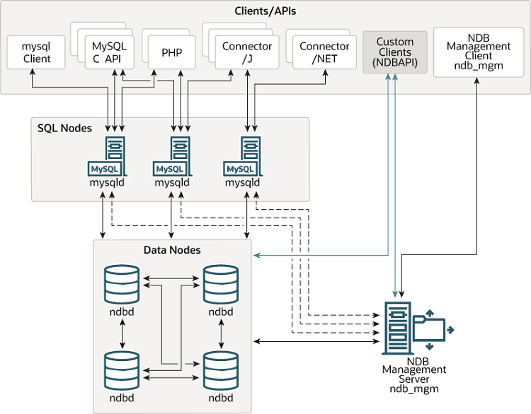
    An NDB Cluster consists of a set of computers, known as hosts, with each one running one or more processes. These processes, known as nodes, may include MySQL servers (for access to NDB data), data nodes (for storage of the data), one or more management servers, and possibly other specialized data access programs. To assure the shared-nothing standing you will need a lot of seemingly redundant hardware to avoid any one piece of being a point of failure.  But if you want 99.999% down time you need to pay for the redundancy as you send your data between servers and data centers. 

    The data stored in the various data nodes for NDB Cluster can be mirrored. The cluster can handle failures of individual data nodes with no other impact than that a small number of transactions are aborted due to losing the transaction state, so write your applications so that they expect to handle transaction failure and retry commits if needed.

    So other than the cost of the hardware, the cost of the networking gear, the salary for some smart folks to run operations,  you really should get an enterprise subscription to get access to MySQL Enterprise Monitor to watch the various components.  

    NDB Cluster is missing some features found in the mainstream MySQL server such a index prefixes, savepoints/rollbacks are ignored, no generated columns, and statement based replication only among others.

    This is your option if you need to be able to have less than 27 minutes of down time a year or really want synchronous replication.

MySQL InnoDB Cluster

    MySQL InnoDB Cluster provides a complete high availability solution for MySQL servers. You use the MySQL Shell which includes the AdminAPI which enables you to easily configure and administer a group of at least three MySQL server instances to function as an InnoDB Cluster. Each MySQL server instance runs MySQL Group Replication, which provides the mechanism to replicate data within InnoDB Clusters, with built-in failover.

  

    You application communicates through a copy of MySQL Router which is a lightweight Level 4 proxy.  MySQL Router then forwards your queries to the cluster.  In the above example we have two machines answering SELECT or read queries only and another server that can handle any query.  The router decides who gets what, will load balance, and works with the cluster machines to avoid problems.  If one of the machine goes offline, Router and the remaining machines will automatically handle the issue but once again make sure your application checks return codes so it can retry a commit.

    InnoDB Cluster is built on MySQL Group Replication which provides a distributed state machine replication with strong coordination between servers. The servers coordinate themselves automatically when they are part of the same group. The group can operate in a single-primary mode with automatic primary election, where only one server accepts updates at a time or for more advanced users the group can be deployed in multi-primary mode, where all servers can accept updates, even if they are issued concurrently. This power comes at the expense of applications having to work around the limitations imposed by such deployments.

    There is also a built-in group membership service that keeps the view of the group consistent and available for all servers at any given point in time. So servers can leave and join the group and the view is updated accordingly. 

    A really cool feature to InnoDB cluster is a plug-in that allows a new machine to be fully loaded with data from a donor machine by making it a clone of the donor.  Very fast, low fuss, and a new machine joining the cluster is fully populated with data.

    MySQL ReplicaSet

    MySQL ReplicaSet is the newest of these offerings with many of the benefits of InnoDB cluster but mainly lacking automatic fail over if the primary stops for some reason.  If you need the high availability, automatic fail over you want InnoDB cluster. But if you have simpler needs and do not occasionally mind promoting a secondary to primary, then you may want ReplicaSet.

    ReplicaSet is MySQL 8.0 only, is GTID only, only supports Row Bases Replication, does not allow replication filters, and there is no automatic fail over.  So if you needs are simpler this is a step up from generic replication and highly recommended due to the Clone plug-ins ability to bring a new node online so quickly.

    Mixes

    You can replicate from NDB or InnoDB Cluster to regular semi/async MySQL servers. So if you want the power of InnoDB cluster but want a safe server out of the clusters for backups or analytics.  

    So What Do I Choose?

    This depends on your needs. Ferraris, I am told, are wonderful cars but they are not made to be dump trucks, fire engines, or low cost grocery getters.

    If you can live with the limitations of NDB need to replicate a) between data centers, b) have minimal down time, c) and have the budget to support a&b then I recommend NDB cluster.  I do know of folks replication between data centers with InnoDB Cluster or generic replication too but NDB was designed to do this all with the minimal down time.

    Need high availability with automatic fail over?  InnoDB cluster.

    Or is your replication need not as sophisticated? Then I recommend ReplicaSET.

Which Account Belongs to Whom or a GCOS Field Equivalent for MySQL Accounts

Last week I received an urgent email asking to move the time of  my performance review up a few hours. And the email sender was not in my management structure and was someone unfamiliar to me. Being a former  Xerox employee, I checked my others emails for notice of a reorganization.  Then I realized the person in question was seeking the other David Stokes at Oracle.  Yup two of us with the same name at the same company. Whew!

Coincidentally MySQL 8.0.21 added a new ability that allows you to store information about an account similar to the way the GCOS field is supposed to be used for in the UNIX/Linux world. Back in time many decades ago, account names were limited in length and the GCOS field was populated with the account's user name, office room number, office phone number, and some other relevant information.  This was the way the system administrator could contact the individual using the account directly. 

The mysql.user table has evolved to 51 fields but only as of 8.0.21 did you have a way to record who was actually using the account.  Or let others know why the accounts exists or other meta data about the account.

For an example I created an account and added a comment about the account.

CREATE USER 'dstokes'@'localhost' 
IDENTIFIED by 'S3cr3t!'  
COMMENT '{ "user" : "Dave"  }';

And the information is stored in a column named User_attributes. 

select User_attributes from user WHERE User='dstokes'\G
*************************** 1. row ***************************
User_attributes: {"metadata": {"comment": "{ \"user\" : \"Dave\"  }"}}
2 rows in set (0.0010 sec)

or you can use the word ATTRIBUTE in the place of the keyword COMMENT.  We do use 'comment' someplace else in the world of Structured Query Language so I would personally prefer ATTRIBUTE in this case.

CREATE USER 'jack'@'localhost' 
IDENTIFIED BY 'XXX123!!!' 
ATTRIBUTE '{ "test" : "yes" }';

Cool, eh?

ALTER USER supporst both keywords.

alter user 'jack'@'localhost' 
ATTRIBUTE '{ "foo" : "Example" }';
SELECT User_attributes from user where User='jack';
+-------------------------------------------------+
| User_attributes                                 |
+-------------------------------------------------+
| {"metadata": {"foo": "Example", "test": "yes"}} |
+-------------------------------------------------+

And please note that reusing a key updates the content. Here I reuse 'foo' and the contents are updated.

alter user 'jack'@'localhost' 
ATTRIBUTE '{ "foo" : "Example revised" }';

SELECT User_attributes from user where User='jack';
+---------------------------------------------------------+
| User_attributes                                         |
+---------------------------------------------------------+
| {"metadata": {"foo": "Example revised", "test": "yes"}} |
+---------------------------------------------------------+
1 row in set (0.0005 sec)


Please remember that the JSON data type column is limited to a gig of data so you can not go too crazy recording information.  But please do start adding some account meta data to help identify your accounts.

Oracle MySQL Virtual Event: Upgrading to MySQL 8.0

Be sure to register for the July 29th  Oracle MySQL Virtual Event: Upgrading to MySQL 8.0! 

Join MySQL's first virtual conference and discover how upgrading to MySQL 8.0 will improve your application performance.  Agenda for the day:

8:00 – 9:00am PDT         Best Practice Tips | Upgrading to 8.0 (LeFred)

9:00 – 10:00am PDT       MySQL 8.0 Through the Eyes of the MySQL Support Team (Megha)

10:00 – 11:00am PDT     Customer Insights from UC Irvine

11:00 – 12:00pm PDT     MySQL 8.0: Indexes, Histograms and Other Ways to Speed Up Your Queries (Dave Stokes)

12:00 – 1:00pm PDT       Transforming Your Application with MySQL 8.0 (Michael Marx)